7575_RefCru

Usamos el método de mínimos cuadrados para sistemas inconsistentes para encontrar una nueva regla de asignación para problemas de racionamiento y excedentes. En particular, estudiamos problemas de asignación considerando diferentes prioridades para satisfacer las demandas de los agentes, lo que influirá en cómo se lleva a cabo la distribución. La nueva regla de distribución se propone eligiendo diferentes productos internos definidos en álgebra lineal y proporcionando fórmulas explícitas para la asignación de recursos a los agentes. Además, ilustramos cómo puede recuperar diferentes reglas de asignación definiendo adecuadamente las prioridades. Como aplicación del problema de racionamiento con agentes prioritarios, se consideran datos reales para la asignación de policías en los estados de México. En este ejemplo, los agentes representan a los estados de México, y sus prioridades se establecieron con base en la incidencia delictiva. Además, calculamos y comparamos la distribución de recursos dada por las reglas clásicas de asignación y el porcentaje de pérdida obtenido con cada una.

PALABRAS CLAVE

Problemas de asignación; método de mínimos cuadrados; agentes prioritarios.

ABSTRACT

We use the least-squares method for inconsistent systems to find a new allocation rule for rationing and surplus problems. In particular, we study allocation problems considering different priorities to satisfy the agents’ demands, which influence how the distribution is carried out. The new distribution rule is proposed by choosing different inner products defined in linear algebra and providing explicit formulas for assigning resources to the agents. Moreover, we illustrate how it can recover different allocation rules by adequately defining the priorities. As an application of the rationing problem with priority agents, we consider real data for allocating police officers in the states of Mexico. In this example, the agents represent the states of Mexico, and their priorities were established based on the criminal incidence. Also, we compute and compare the resource distribution given by classic allocation rules and the percentage of loss obtained with each one.

KEYWORDS

Allocation problems; Least;squares method; Priority agents.

Clasificación JEL: C02, C79.

MSC2010: 91B32, 91A80.

1. Introduction

In the administrative sciences, problems of goods or resource distribution among agents frequently appear. A typical situation is when each agent demands a certain amount of resources. Depending on the available resource, one may find three cases: when it is less than, greater than, or equal to the demand. The first case is called a resource rationing problem since the demands exceed the available resource and cannot be satisfied. The most common rationing problem in the literature is the so-called Bankruptcy problem, where the solutions must be non-negative, and no agent can obtain more than was demanded. When these characteristics of the solution are not fulfilled, we say that we have a rationing problem, allowing other types of solutions. In these types of problems, an agent can be assigned more than demanded or even to provide from his resources, depending on the priority factors, which could imply a redistribution of resources. We call the second case a surplus problem because it seeks to distribute the surplus or excess of the available resource after the demand of each agent is satisfied. It implies that each agent receives at least what was demanded. The third case is trivial since the available resource equals the demands of the agents: each agent obtain the demanded amount, and the resource will be used completely. Thomson (2003) has a fascinating treatise on the distribution problems of both rationing and surplus, giving characterizations of the solutions to the problems. They also considered “whole” distribution problems and non-transferable utility problems.

Indeed, the most interesting case is the rationing one. If no agent obtains his total demand, deciding how the resource is divided is essential. In particular, allocation rules for the bankruptcy problem are abundant in the literature (Ólvera-López et al., 2014; O’Neill, 1982). In particular, bankruptcy problems were studied from the point of view of game theory (Guerrero et al., 2006) and the solutions were obtained by applying concepts from cooperative game theory. The authors provided the conditions to make an allocation rule for bankruptcy equivalent to a game-theoretic rule.

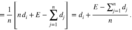
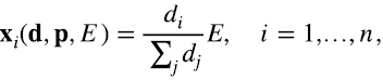
Let us backtrack to the general setting of allocation problems. Such problems are defined as a pair , where d=(d1,...,dn) is called the demand vector, di≥0 denotes the demand of agent i, f = 1,...,n, while E > 0 represents the available amount of a perfectly divisible resource. Given a (d, E) problem, a solution or distribution rule is an n–vector x(d, E) where the components are indexed by the agents and . In the literature, there are several rules for allocating resources. Indeed, it depends on the type of problem, but our approach is to set a system of n+1 linear equations and n unknowns as follows (1.1) (1.2)

(1.1)

(1.2)

where equations (1.1) are called “demands” and equation (1.2) is called the “efficiency equation”. Notice that the surplus case corresponds to , while the rationing case is when 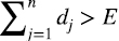. For both cases, the system given by equations (1.1) and (1.2) is inconsistent meanwhile in the case 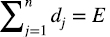, the system has the trivial solution. Notice that the solutions of the system, equations (1.1) and (1.2), are not restricted to being non-negative or assigned less or equal to his demand, i.e., we have a rationing problem. We should distinguish the problem that we are dealing with, the bankruptcy problem. However, conditions can be set in the demands so that the obtained solution satisfies the bankruptcy problem. To solve this problem, the least-squares method (LSM) for inconsistent systems appears naturally in this context to obtain an approximate solution. This method has been used not only in different areas, such as statistics (Casella and Berger, 2021), or linear algebra (Margalit et al., 2017), but to solve allocation problems set as incompatible or inconsistent systems (Cruze et al., 2014). One problem with the last approach is that the efficiency equation is not necessarily satisfied because the LSM approximates the solution. However, it is desirable to have an allocation rule that ultimately divides the resources, insufficient or exceeded, i.e., to prioritise the efficiency equation. A heuristic way to prioritise an equation is to repeat it several times. Let us say that we repeat k-times times the efficiency equation. Therefore, we have a system of n + k equations whose least-squares solution gives more weight to the efficiency equation. In this way, we apply the same LSM to a more extensive linear system of equations.

In this paper, we establish the relation between the repetition of an equation and a specific inner product considered in the LSM, which reformulates this problem. The idea of using modified inner products has been applied in LSM to find an optimal set of vectors to minimise the sum of the squared norms of errors (Eldar, 2002).

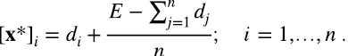
This approach corroborates, by using a suitable inner product, that if we repeat the efficiency equation k-times times the least-squares solution converges to 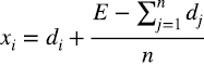, as k tends to infinity. This solution has a simple economic interpretation: each agent receives what it demands, plus or minus, an n–th of the deficit or surplus, respectively. This rule is similar (under certain conditions) to the one known in the literature as the Constrained Equal Loss rule (Lorenzo, 2010), prioritising to the agents with higher demand. Other characteristics of this rule are consistency, exclusion, composition up, composition down, and symmetry, which have been proven in the bankruptcy literature (Herrero, 2003). Let us say that repeating rows implies that we have trivial correlated data where methods, such as the generalised weighted LSM, deal with this type of data (Strutz, 2011).

Additionally, we generalise this rule to consider priorities for the resource distribution among the agents, first-priority agents, second-priority agents, and others. We show that if the equations concerning priority agents are repeated in proportion to their priorities, the LSM solution converges to a solution that satisfies their respective preferences. Moreover, we present a procedure to set priorities to recover different distribution rules (solutions) reported in the literature (Moulin, 2000).

This article is organised as follows. In Section 2, we provide a background on the LSM and some linear algebra concepts, which allow us to generalise the LSM by using different choices of inner products. In Section 3, we establish a link between the repetition of an equation and the M-inner product, and two numerical examples are presented. In Section 4, we develop a new distribution rule for allocation problems considering priority agents. In Section 5 we show some interesting properties satisfied by the distribution rule and illustrate how it is possible to recover different allocation rules just by setting the priorities appropriately. Later, we present an application of the rationing problem with priority agents considering real data in Section 6. Finally, in Section 7, we conclude with some comments.

2. The LSM and linear algebra concepts

Let us consider a system consisting of equations (1.1) and (1.2) which can be written in matrix notation as (2.1)

(2.1)

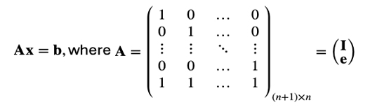
where I is the identity matrix of dimension n x n, e is a row vector of n ones, and b=(d1, d2,...,dn, E)T. Recall that in the rationing and surplus allocation problems, the system is inconsistent, i.e., Ax ≠ b, for all . Then, we search for an approximate solution according to the following definition.

Definition 2.1 Let A be a matrix of dimension m x n and . A least squares solution of the matrix equation Ax = b is a vector such that , for all , where d(v,w) = | | v - w | | is the euclidean distance between the vectors v and w.

In mathematics, there is a precise definition of “distance,” and the least-squares solution makes sense regardless of the chosen distance. The way to define a distance compatible with the linear structure is via an inner product, we will now recall.

Definition 2.2 An inner product on a real vector space V is a function with the following properties:

1. (Positivity) <v,v> ≥ 0 for all with equality if and only if v = 0.

2. (Symmetry) <v,u> = <u,v> for all.

3. (Bilinearity) < λv1 + βv2, u> = λ <v1, u> + β <v2, u> for all and .

The definition of inner product <-,-> on V induces a norm of a vector : | | v | |2 : = <v,v>, and a distance function , d(v,u): = | | v - m | |. Also, the inner product defines the orthogonality relation on V, where we say that the vectors and u in v are orthogonal if <v,u> = 0.

The prime example of an inner product in is the usual dot product in : v · u:=vTu=vTIu, where I is the identity matrix. However, this is not the only one. Note that the definition of the inner product is satisfied if any real symmetric positive definite matrix M replaces the identity matrix. Recall that an m x m real symmetric matrix M is positive definite if vTMv > 0, for all non-zero vectors . In this case, we have a new inner product which we call the M-inner product.

Definition 2.3 Let M be a m x m real positive definite matrix, we define the M-inner product as <v,u>M = vTMu, for .

A classical result states a bijection between the set of inner products in and the collection of m x m positive definite matrices, see for example Hoffman et al. (1973; Ch.8). As it will be explained later, the matrix M plays a central role in determining the priorities. Let us look at one example of the M-inner product.

Example 2.1 In , the positive definite matrix defines the M-inner product <v,u>M=v1u1 + v2u2 + 2v3u3, while the inner product corresponds to the identity matrix. Note that with this inner product the canonical basis {e1,e2,e3} remains orthogonal, i.e., <ei,ej>M = 0fori ≠ j, but it is no longer orthonormal because <e3,e3>M = 2.

Let us remark that if V is a finite-dimensional real vector space and is a linear subspace, then each choice of inner product < -,- >M determines an orthogonal complement such that V can be written as the direct sum, , along with the corresponding orthogonal projection .

Along these concepts, recall that column space of A, Col(A), is the set of all vectors c so Ax = c is consistent. In other words, Col(A) is the set of all vectors of the form Ax. In the setting of Definition 2.1, it is true that for any vector , there is one and only one vector in the subspace W : Col(A), which minimises the distance | |b-Ax| |M. It is given by the orthogonal projection, i.e., . Note that the vector varies with each choice of M. Therefore, a least-squares solution of Ax=bis a solution of the consistent equation (Margalit et al., 2017). Finding an explicit formula for the least-squares solution, as described in the following proposition.

Proposition 2.1 Let A be a matrix of size m x n with real entries, and M a positive definite matrix of size m x m. A vector is a least squares solution of the equation Ax=h with respect to the M-inner product if and only if it satisfies the following equation (2.2):

(2.2)

Proof. Let be the column space Col(A) as before. We know that x is the least-squares solution if and only if , and this is equivalent to saying that the vector v: = Ax-h is in the orthogonal complement of W in , where .

Now if c1,..., cn denote the column vectors of A, then the vector v is uniquely determined by the equations <c1,v>M = 0,..., <cn,v>M = 0. Since <cj,v>M = cjTMv, for j = 1,..., n, we can write up all the equations in a matrix form by ATMv=0.

Rewriting v by its definition, we obtain that, 0 = ATMv = ATMb (Ax-b), or equivalently ATMAx = ATMb. Q.e.d.

Note that if Ax = b is consistent, then so that a least-squares solution is the usual one. We call the M-Least Squares Method (M-LSM) to the solution where the distance function is given by the norm induced by the M-inner product, see Definition 2.2. There is a case where the M-LSM solution can be explicitly computed.

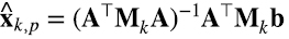
Theorem 2.1 In the setting of Proposition 2.1, the system Ax =b, has a unique least-squares solution with respect to the M-inner product if and only if the columns of A are linearly independent. In this case, the M-LSM solution is given by (2.3)

(2.3)

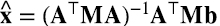
Proof. We know that x is a least-squares solution if and only if its image Ax is equal to the orthogonal projection of b. This solution is unique if and only if the linear transformation associated with A is injective, which is equivalent to A having linearly independent columns. All that is left to prove is that, in this case, the matrix ATMA is invertible.

Note that for any we have that 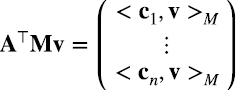which tells us that the kernel (nullspace) of ATM is equal to the orthogonal complement of the column space of A.

For we have that and since A is injective then w ≠ 0 implies that Aw ≠ 0. But since 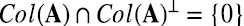, we have that Aw is not in the kernel of ATM. In particular, the linear transformation associated with the matrix ATMA is injective, i.e., it has linearly independent columns, but since it is a square matrix, this is equivalent to being invertible. Q.e.d.

Remark 2.1 Recall that the key concept in M-LSM is orthogonality, which depends on the definition of the inner product of two vectors in . As we mentioned before, the euclidean distance is associated with the usual dot product, and the corresponding matrix is the identity I. In this case equations (2.2) and (2.3), for the usual LMS, become (2.4),

(2.4)

respectively, which is how we usually find them in the literature.

3. M-LSM and allocation problems

In this section, we provide a Theorem where the efficiency equation is prioritised in allocation problems, solved by the LSM, which led us to an allocation rule that we called the LSM rule. Also, we establish a link between the LSM resolution of this linear system and its solution using an M-inner product. These two results are fundamental to proposing a new and more general allocation rule.

Let us begin by applying these results to allocation problems given by equations (1.1) and (1.2), but repeating the last equation k-times times to give it a certain priority, i.e., xi = di, i=1,...,n, (3.1)

(3.1)

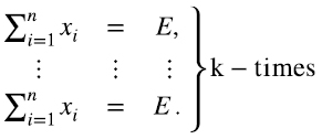
In matrix notation, this system can be written as Akx =bk, where (3.2)

(3.2)

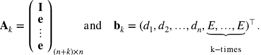
When the column vectors of Ak are linearly independent, or Ak has a complete rank, it is possible to obtain its limit by taking k to infinity. Note that this implies that the number of equations tends to infinity.

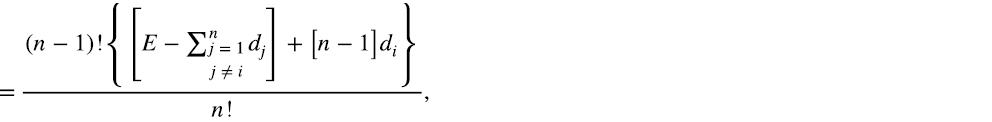
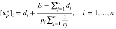
Theorem 3.1 Let Ak be a complete rank matrix as defined in (3.2), Akxk=bk the system of equations given by (3.1), and the LSM solution for this system. Then, converges to x* k → ∞ as, whose i–th element is given by (3.3)

(3.3)

We call this equation LSM rule.

Proof. We aim to find the i–th component of the vector denoted by . From Remark 2.1, which refers to the usual LSM, and the assumption that the columns of Ak are linearly independent, the solution of system (3.1), , is given by equation (2.4), .

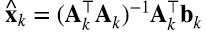Firstly, we have the matrix AkTAk is of dimension n x n, whose i j–th element is given by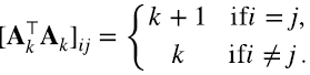

The element i j of the inverse of this matrix is given by .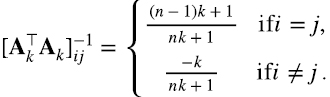

Multiplying the computed inverse by AkT, we get .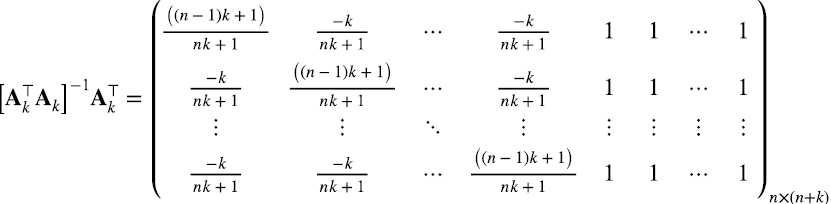

To calculate the i-th term of , we multiply this matrix by the column vector bk, i.e.,

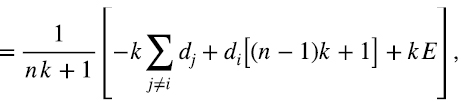
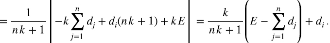
Now, we show the convergence of to [x*], as k tends to infinity. We have that (3.4)

(3.4)

since (3.4) can be made arbitrarily small with large enough k, then we have that converges to a vector x* whose i–th component is given by (3.3). Q.e.d.

Note that this theorem shows that 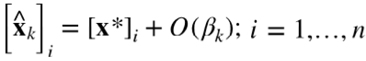, where 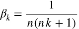, which is the rate of converge of . The solution found in Theorem 3.1 is equivalent to the Constrained Equal Loss solution in the bankruptcy context when allocations are non-negative (Lorenzo, 2010). Note that we are assuming that there are no priorities among the agents. The only priority given is to the efficiency equation.

Remark 3.1 In the surplus problem, the solution can also be obtained analogously to the recursive formula used in bankruptcy problems (Guerrero et al., 2006). Let us consider the n permutations. In each permutation, the agent that first appears (the first to arrive) is allocated the surplus, assuming that the rest of the agents are allocated their respective demand. Then, we average the n allocations of the agents, and thus, the agent i obtains: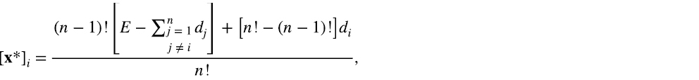

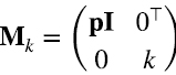
To finalise this section, we discuss the relationship between the repetition of the efficiency equation (1.2) and the M-inner product. Recall that the system without repetitions of the efficiency equation is given by equation (2.1). On the other hand, let us define the matrix Mk of dimension (n+1) x (n+1) , as in Proposition 2.1, (3.5)

(3.5)

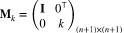
where k is the number of repetitions of the efficiency equation, 0 is a row zero vector of dimension n, and I is identity matrix of size n x n.

The M-LSM solution given by Theorem 2.1, equation (2.3) is given by 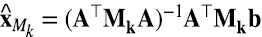which is obtained using the M-inner product, Definition 2.3. It is easy to see that (ATMkA)-1 = (AkTAk)-1 and ATMkb = AkTbk, therefore 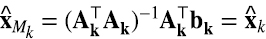. This is very useful because instead of working with linear systems of high dimension (large k), we only have to modify the [(n+1),(n+1)]–th element of the matrix Mk given in (3.5). In particular, the M-LSM solution of Theorem 2.1 coincides with the solution of Theorem 3.1, and so we have that .

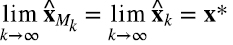We will come back to this in a more general setting in Section 4.

In the next subsection, we illustrate the convergence of the M-LSM solutions for rationing and surplus problems.

3.1 Examples of rationing and surplus problems

In the following two examples of allocation problems, we repeat k–times the efficiency equation to show that the LSM solution tends to the equal loss rule for both rationing and surplus cases.

Example 3.1 Let us consider the rationing problem ((60,40,30);100) where the demand vector for the 3 agents is d=(60,40,30) and the available resource is E=100.

The associated system of linear equations to be solved by the M-LSM is the following: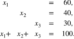

This is a rationing problem since the total demand is 130 while the resource is only 100. In Table 3.1, we show the M-LSM solutions considering different values for k repetitions of the efficiency equation. When k=1, we have the usual LSM solution. Note that none of the equations of the system is satisfied. As the value of k increases, the efficiency equation is closer to being satisfied.

Table 1

Table 1. Solutions of the rationing problem ((60,40,30);100).

k	x1	x2	x3	x1+x2+x3
1	52.50000	32.50000	22.50000	107.50000
10	50.32258	30.32258	20.32258	100.96774
100	50.03322	30.03322	20.03322	100.09967
1000	50.00333	30.00333	20.00333	100.01000
10000	50.00033	30.00033	20.00033	100.00100

Let us recall this limit is given by equation (3.3) of Theorem 3.1, thus [x*]1=50,[x*]2=30 and [x*]3=20. Notice that this solution coincides with the bankruptcy one, and the demand loss is 10 for each agent.

Example 3.2 In this example, we apply the results to a surplus problem ((60,40,30);20) where the available resource is E=200. In Table 3.2, we present the solutions of this system for different values of the repetition of the efficiency equation, k. Note that the efficiency is also satisfied as k tends to infinity.

Table 2

Table 2. Solutions of the surplus problem ((60,40,30);200)

k	x1	x2	x3	x1+x2+x3
1	77.50000	57.50000	47.50000	182.50000
10	82.58065	62.58065	52.58065	197.74194
100	83.25581	63.25581	53.25581	199.76744
1000	83.32556	63.32556	53.32556	199.97667
10000	83.33256	63.33256	53.33256	199.99767

4. Allocation problems with priority agents

An interesting case in allocation problems is considering different priorities to satisfy the demands of the agents, which are characteristics that agents may have or possess and that will influence the way the distribution is carried out. In contrast to the previous section, where the priority was only the efficiency equation, in this one, the priorities can be set for several equations and using the M-LSM to solve them. Let us focus on solving the system Ax=h according to Theorem 2.1 where M is a matrix is given in a more general form (4.1)

(4.1)

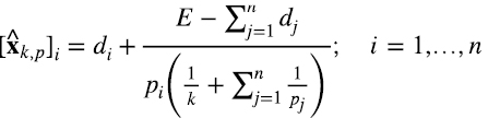
where p=(p1,...,pn), and Pi ≥ 1 is the priority of the agent i, . Let us say that those priorities, p, are a generalisation of the repetitions of equation i, but they are no longer required to be a natural number. Moreover, if pi<pj, we say that agent i has priority over agent j. In the following Corollary, we give a closed formula for the allocated amount each agent receives depending on its priority which is also one of our main results.

Theorem 4.1 Let Axk,p=b be the system of equations resulting of an allocation problem given in equations (1.1) and (1.2), and let Mk as in (4.1). Then, the i–th element of the M-LSM solution of this system, , is given by (4.2).

(4.2)

Proof. From Theorem 2.1, we have that (4.3).

(4.3)

To compute the i–th element of this solution, we first obtain the i j–th element of the n x n matrix ATMkA,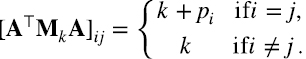

Now, we can find the inverse matrix using the adjoint matrix as follows, where and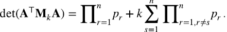

On the other hand, since the i–th coordinate of ATMkb is given by [ATMkb]i=pidi+kE, then

Q.e.d

Remark 4.1 In terms of allocation problems, it is necessary for the efficiency equation to be satisfied, which can be achieved by taking the limit of the equation (4.2), as k tends to infinity. Therefore, converges to xp* as k→∞, whose i–th element is given by (4.4).

(4.4)

Let us call this the Priority M-LSM rule.

5. Properties of the M-LSM rules and its relationship with other distribution rules

In this section, we describe some properties that the Priority M-LMS rule satisfies and recover existing allocation rules by tuning the agents’ priorities and applying the M-LSM rule.

Firstly, we introduce some notation in the context of the allocation problem. Notice that the solution given by (4.4) is a function where d, p and E are the demand vector, the priority vector, and the resource, respectively. Now, let us describe some interesting properties that satisfy the M-LSM rule with and without priorities:

Property 1. The solution x(d,p,E) satisfies the scale invariance property if X(λd,p,λE)=λx(d,p,E)for all ≥0

Property 2. The solution x(d,p,e) satisfies the equal treatment property if di=dj and pi=pj, then xi(d,p,E)=xj(d,p,E).

Property 3. The solution x(d,p,E) satisfies the monotonicity property if di ≥dj and pi=pj, then xi(d,p,E)≥xj(d,p,E)

Property 4. The solution x(d,p,E) satisfies the efficiency property if

Property 5. The solution x(d,p,E) in the case that satisfies the priority property if pi>pj and xj(d,p,E)=dj, then xi(d,p,E)=di.

Proposition 5.1 Solution (4.4) satisfies scale invariance, equal treatment, monotonicity, efficiency, and priority properties.

Proof. For the scale invariance property note that for all i=1,...,n and λ≥0,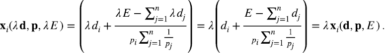

If pi=pj, equal treatment and monotonicity properties are trivial. For the efficiency property observe that,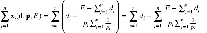

For the priority property, assume that and let us proceed by contrapositive. Observe that if xi(d,p,E)<d, then 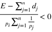. Since pi>pk , we have

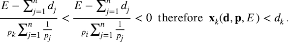
Q.e.d.

Corollary 5.1 The allocation rule given in (3.3) satisfies scale invariance, equal treatment, monotonicity, and efficiency properties.

On the other hand, it is important to observe that it is possible to recover classic distribution rules that can be found in the bankruptcy literature:

1. m–Agent Priority LSM Rule: If pi→∞ for some i, and later k→∞, then xi(d,p,E)=di which means that agent i has the greatest priority, so he obtains his total demand. If the rest of the agents have the same priority, i.e., pj=1, for j≠i, then substituting in the M-LSM rule, equation (4.4), we obtain where 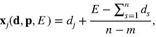m denotes the number of high priority agents, m<n. It means that the method takes for granted equation i and works only with the other equations.

2. Proportional Rule: If 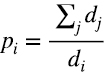, for i=,...,n, the equation (4.4) is given by (5.1),

(5.1)

which is the solution of the proportional allocation rule Guerrero et al., (2006). This rule follows because we set the priorities as a proportion of each agent’s demand.

3. Equal Allocation Rule: If we have that , and , then we recover the Equal Allocation solution Guerrero et al., (2006) given by 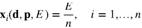, where all agents receive the same amount.

4. Constrained Equal-Loss Rule: In this case, the solution is given by fi=max{di-λ,0}, i=1,...,n, where λ is such that . This rule was defined in Guerrero et al., (2006). If xi(d,p,E)≥0 then fi=xi(d,p,E)≥0, i=1,...,n and its solution is given by equation (3.3). We can recover this solution taking pi=1for all i, in equation (4.4). We request the solution to be positive because a negative one would imply that some agents do not obtain their demands, and they will have to contribute to pay other agents’ demands.

6. Application: A proposal for the police force distribution in Mexico

This section presents an application to a real police force distribution in Mexico according to different agents’ priorities. In this case, the agents represent the states of Mexico, and their priorities were established based on the criminal incidence. We illustrate how M-LSM can recover classic allocation rules and compares the percentage of loss obtained with each one.

It is well known that criminal incidence in Mexico is a significant problem. However, it is not the same for the 32 states of this country, according to Public Safety and Justice, 2018 from (INEGI, 2022b). Based on this fact, we investigate the real allocation of the police force and propose a new distribution for the states considering the criminal incidence to prioritise the allocation of each state.

The real number of on-duty police officers is given by the Real State Force (RSF) from (Secretaría de Seguridad y Protection Ciudadana Diario Oficial, 2021). Summing up this data, the total number of police officers in Mexico is E=230,217. On the other hand, it is known that there is a deficit of more than 100,000 police officers in the country (INEGI, 2022a), 42 % of the state preventive police forces fail to meet the minimum standard of 1.8 police officers per 1,000 inhabitants (Secretaría de Seguridad y Protection Ciudadana Diario Oficial, 2021). We can calculate the recommended police force for each state (agents’ demand) according to , where the population of each state was taken from the National Institute of Statistics and Geography (INEGI, 2021).

We consider the population older than 20 years since we are interested in adults, and the age intervals given by the INEGI are reported in periods of five years. Thus, the required number of police officers in Mexico is approximately .

Our allocation method considers the agents’ priorities in several ways to fulfill this demand. Moreover, the allocation results will depend on this selection, as described in Section 5. For this reason, we consider three different ways of assigning priorities:

1. LSM rule: By setting pi=1, for all i=1,...,32, we assign to each agent the same priority.

2. Proportional rule: If (see equation (5.1)) for i=1,...,32, i.e., the priority of the agents is proportional to their demand.

3.Priority M-LSM rule: As an example, we consider the criminal incidence to set the values of pi to show the versatility of the method, but other criteria could be applied. We chose pi as the total number of crimes committed by the population aged 18 and over, per 100,000 inhabitants, for each state i. We consider the data from the National Survey of Victimization and Perception of Public Safety Public Safety and Justice 2018 (INEGI, 2022b).

In Table 2, we present the Mexican population aged 20 years and older, the real number of police officers, and the police demands for each state. Also this table shows that the set of priority values, pi, which correspond to the cases mentioned above.

Table 3

Table 3. Population data, real number of police officers (RSF), demand, and priorities.

State of Mexico	Pop. 2020	RSF	Demand	LSM	Prop.	Priority
Aguascalientes	906937	599	1632.4866	1	91.7138	36500
Baja California	2566859	925	4620.3462	1	32.4048	42725
Baja California Sur	532083	375	957.7494	1	156.3265	28377
Campeche	606811	1280	1092.2598	1	137.0751	26466
Coahuila	2047048	1646	3684.6864	1	40.6335	24813
Colima	495609	913	892.0962	1	167.8312	28376
Chiapas	3219331	6073	5794.7958	1	25.8373	19409
Chihuahua	2465574	2024	4438.0332	1	33.736	28622
Ciudad de México	6897156	38631	12414.8808	1	12.0598	69716
Durango	1152581	764	2074.6458	1	72.1673	22586
Guanajuato	3967101	2911	7140.7818	1	20.9671	38067
Guerrero	2164767	3184	3896.5806	1	38.4238	43051
Hidalgo	2015711	2948	3628.2798	1	41.2652	25987
Jalisco	5476852	5324	9858.3336	1	15.1873	40543
México	11385459	16815	20493.8262	1	7.3057	51520
Michoacán	3039249	3236	5470.6482	1	27.3682	22999
Morelos	1335367	1180	2403.6606	1	62.289	45312
Nayarit	799154	914	1438.4772	1	104.0834	23670
Nuevo León	3912966	5384	7043.3388	1	21.2572	27805
Oaxaca	2617078	3575	4710.7404	1	31.783	26221
Puebla	4189703	3500	7541.4654	1	19.8531	37647
Querétaro	1580039	784	2844.0702	1	52.6434	32756
Quintana Roo	1232014	1465	2217.6252	1	67.5144	33243
San Luis Potosí	1840078	2693	3312.1404	1	45.2039	32342
Sinaloa	2016233	1516	3629.2194	1	41.2545	29507
Sonora	1962552	1223	3532.5936	1	42.3829	50861
Tabasco	1539429	4552	2770.9722	1	54.0322	36546
Tamaulipas	2355594	4136	4240.0692	1	35.3111	25368
Tlaxcala	852929	1294	1535.2722	1	97.5212	40336
Veracruz	5416658	5911	9749.9844	1	15.3561	25350
Yucatán	1569474	3412	2825.0532	1	52.9978	26462
Zacatecas	1020268	1030	1836.4824	1	81.5263	26670

In Figure 1, we present the results of applying of the priority LSM rule, equation (4.4), to obtain the number of police officers allocated in each state of Mexico using the three different value sets of pi. This figure shows that the allocation made by the different distribution rules is similar for some states but not for others.

Figure 1

Figure 1. Graphs of the RSF, demand, and allocation solutions of police officers using three types of priorities for each state of Mexico

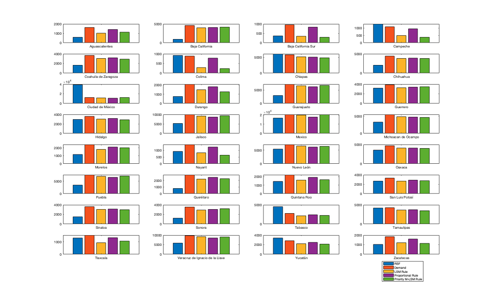
To explain this, let us focus on a particular case such as Campeche, where the police officer demand is high. However, the police officers’ allocation, with and without priority, is low even though the actual RSF exceeds the requested demand. In this state, the criminal incidence is low, which explains the low allocation using the priorities. On the opposite side, the proportional solution is higher in agreement with the size of the population. The resolution without priority is higher than the solution with priorities because it does not consider Campeche State a low-incidence state. Therefore, considering criminal incidence, the allocation can change significantly. Also, from Figure 1, we can see the difference between the demand and the allocation, which we call loss, for each state.

To visualise more easily the difference among the rules, in Figure 2 we present the percentages of loss for each one. As expected, the Proportional rule always gives the same percentage of loss to all the agents (states), approximately 13 %. In contrast, the loss percentage loss for the LSM and the Priority M-LSM can vary abruptly from one state to the other. In this figure, we can also observe that the difference between the percentage of loss is significant for these two rules for most of the states.

With the aim of analysing the new rule, let us focus on the priority M-LSM solution based on the criminal incidence. For this solution, the states with a higher percentage of loss are Colima, Baja California Sur, Campeche, Nayarit, and Durango, while the states with a lesser loss percentage are Mexico, Ciudad de Mexico, Jalisco, Puebla, and Guanajuato.

Figure 2

Figure 2. Percentage of a loss considering the LSM rule, proportional rule, and priority LSM rule for each state of Mexico

Figure 3

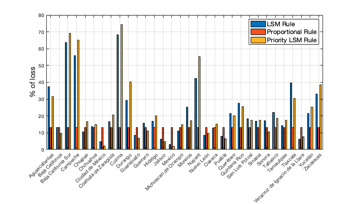
Figure 3: Percentage of loss of the demanded number of police officers and criminal incidence for each state of Mexico

Figure 4

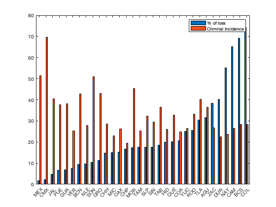
Figure 4 Surplus (positive) and deficit (negative) of police officers of RSF according to Priority LSM solution in each state of Mexico

In Figure 3 we present the percentage of loss of the demanded number of police officers in ascending order and the criminal incidence for each state of Mexico. One might expect that the loss percentage is low for a high criminal incidence because the priority was established on this factor. For some states, this occurs, but for other states, do not since the police officer allocation also depends on the demand, which is a linear function of the population of each state. In Figure 4 we show the surplus and deficit of police officers of RSF according to the Priority M-LSM solution in each state. Notice that Mexico City has the highest excess of police officers according to the priority M-LSM rule. Moreover, the surpluses, mainly from Mexico City, are allocated among the states with a deficit. This analysis shows the capabilities of this new rule.

7. Conclusions

In this work, we have provided a new distribution rule for rationing and surplus problems using the least squares method, whose primary results have been mathematically proven through topics of inner products and orthogonality. This new rule was obtained by modifying the inner product associated with the LSM solution (M-LSM), where M is a positive definite matrix of the inconsistent system related to the allocation problem. The solution of this system is generalised by considering priority agents (each agent has some “weight” or priority in the distribution, according to specific characteristics that influence the problem). This extended solution is a generalisation of some distribution rules existing in the literature. To illustrate our results, we have applied the priority M-LSM rule to a real problem, such as allocating the number of police officers in Mexico by prioritising the allocation for the states with the higher criminal incidence. Indeed, we can consider more than just one feature of the states to assign the priority pi and thus find their allocation. This new way of distribution considers more factors that may influence the allocation problem. The full characterisation of this rule will be a matter of future work.

Autor Contributions

Conceptualization, JCMP, AEGF and SEDA; data curation LJRE; formal analysis, JCMP, LJRE, SEDA, RAKC and AEGF; methodology, JCMP, AEGF and SEDA; software, SEDA and LJRE; validation, SEDA, RAKC and LJRE; investigation, LJRE and SEDA; resources, JCMP, RAKC; writing original draft preparation, JCMP, AEGF, SEDA, RAKC and LJRE; writing review and editing, JCMP, AEGF, SEDA, RAKC and LJRE; visualization, SEDA and LJRE; project administration, RAKC and LJRE; funding acquisition, JCMP, SEDA and RAKC. All authors have read and agreed to the published version of the manuscript.

REFERENCES

Casella, G. and Berger, R. L. (2021). Statistical inference. Cengage Learning.

Cruze, N. B., Goel, P. K., and Bakshi, B. R. (2014). Revisiting least squares techniques for the purposes of allocation in life cycle inventory. The International Journal of Life Cycle Assessment 19(10), 1733–1744.

Eldar, Y. C. (2002). Least-squares inner product shaping. Linear algebra and its applications 348(1-3),153–174.

Guerrero, F. M., Hinojosa, M. Á., and Sánchez, F. (2006). Teoría de juegos aplicada a problemas de bancarrota. Contribuciones a la Economía, (2006).

Herrero, C. (2003). Equal awards vs. equal losses: duality in bankruptcy. In Advances in economic design, Springer, Berlin, Heidelberg, pages 413–426.

Hoffman, K., Kunze, R., and Finsterbusch, H. E. (1973). Álgebra lineal. Prentice-Hall Hispanoamericana.

INEGI (2021). Población total por entidad federativa y grupo quinquenal de edad según sexo, serie de años censales de 1990 a 2020. https://www.inegi.org.mx/app/tabulados/interactivos/?pxq=Poblacion_Poblacion_01_e60cd8cf-927f-4b94-823e-972457a12d4b idrt=123 opc=t. Accessed: 2023-08-01.

INEGI (2022a). Identifican déficit de más de 100,000 policas en el país. https://www.eleconomista.com.mx/politica/Identifican-deficit-de-mas-de-100000-policias-en-el-pais-20210504-0014.html. Accessed: 2023-08-01.

INEGI (2022b). Incidencia delictiva. https://www.inegi.org.mx/temas/incidencia. Accessed: 2023-08-01.

Lorenzo, L. (2010). The constrained equal loss rule in problems with constraints and claims. Optimization 59(5), 643–660.

Margalit, D., Rabinoff, J., and Rolen, L. (2017). Interactive linear algebra. Georgia Institute of Technology.

Moulin, H. (2000). Priority rules and other asymmetric rationing methods. Econometrica 68(3), 643–684.

Ólvera-López, W., Sánchez-Sánchez, F., and Tellez-Tellez, I. (2014). Bankruptcy problem allocations and the core of convex games. Economics Research International 2014, 517951.

O’Neill, B. (1982). A problem of rights arbitration from the talmud. Mathematical social sciences 2(4), 345–371.

Strutz, T. (2011). Data fitting and uncertainty: A practical introduction to weighted least squares and beyond. Springer.

Thomson, W. (2003). Axiomatic and game-theoretic analysis of bankruptcy and taxation problems: a survey. Mathematical social sciences 45(3), 249–297.

Secretaría de Seguridad y Protection Ciudadana Diario Oficial (2021). Modelo nacional de policía y justicia cívica. https://www.gob.mx/cms/uploads/attachment/file/542605/DOC_1._MODELO_NACIONAL_DE_POLIC_A_Y_JC.pdf, Last accessed on 2017-11-30.